Mathematics 280A (Fall 2012)

[ Home ] [ Math Dept ] [ UPS


Contents


Course Logistics


Day-by-Day Notes

Day and Date

another line of stuff

I am trying to find out how to type out xtml lang="en-US">

Topics:
Text:
Tomorrow:
Comments:

Monday October 29

Topics: Questions on polar coordinates and graphing; Double integrals in polar coordinates
Text: 13.4
Tomorrow:
Comments:

Friday October 26

Topics: Questions on double integrals and polar coordinates; Area density problems;
Text: 9.1, 9.2
Tomorrow: Questions on polar coordinates and graphing; Double integrals in polar coordinates
Comments:

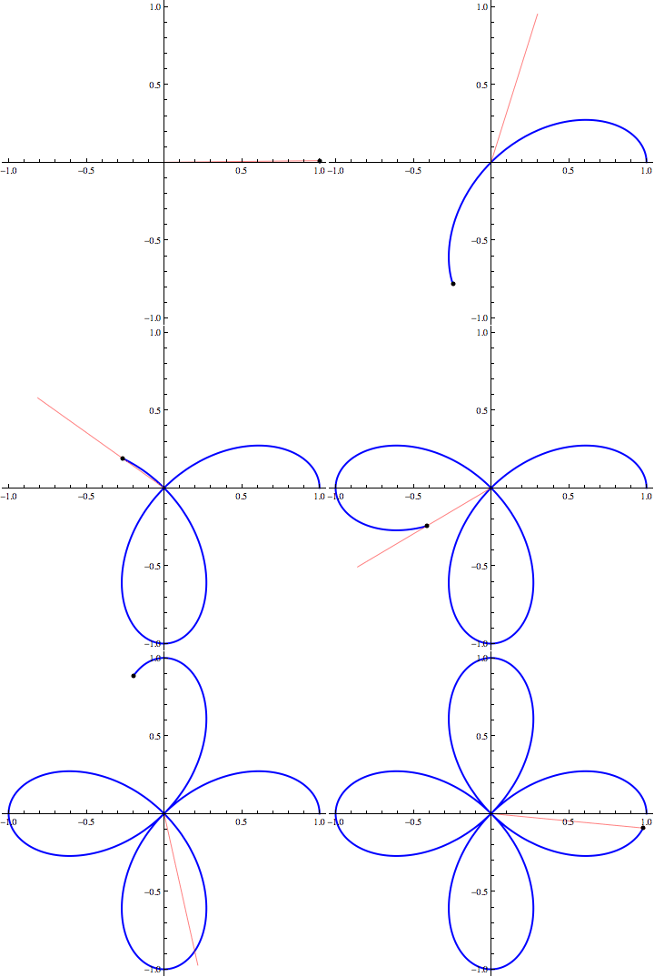
Today, we discussed the basics of polar coordinates and plotting polar curves. The animation below shows the curve r=cos(2θ) being traced out as θ increases. Note that half of the points have negative \(r\) values and hence are being plotted on the ray opposite to the ray specified by θ. Monday, we'll address questions from Section 9.1 and 9.2 problems. If this does not provide you with enough comfort using polar coordinates, we can arrange a time to talk outside of class.

< figure class=center>polar curve animation

Many graphing calculators have a polar graphing feature. On a TI-8X, you can get to this by going to the MODE menu and choosing the option Pol from the list Func Par Pol Seq. If you then go to the Y= menu, you will see r1= where you can enter a formula for a polar curve. On WolframAlpha, you can just type in the polar relation.

The writing exercise is due on Thursday November 1. You should refer to the writing exercise handout and the notes on writing in mathematics for general directions. Also review the paragraph on projects in the course information handout.


Thursday October 25

Topics: Questions on double integrals; Double integrals over general regions (13.2); Polar coordinates and graphing using polar coordinates (9.1, 9.2)
Text: 13.2, Area density problems, 9.1, 9.2
Tomorrow: Questions on double integrals and polar coordinates; Area density problems; Double integrals in polar coordinates
Comments:

Today, we looked at double integrals over non-rectangular regions. To set up an equivalent iterated integral, we need to describe the region with bounds on the cartesian coordinates x and y. If the region is rectangular, we will have constant lower and upper bounds on both x and y. If the region is not rectangular, we will have constant lower and upper bounds on either x or y and at least one nonconstant bound on the other one. The variable with constant bounds must be the outer variable in the iterated integral. In some cases, it is best to split the original region into smaller pieces and to then describe each piece with appropriate bounds on x and y.

The writing exercise is due on Thursday November 1. You should refer to the writing exercise handout and the notes on writing in mathematics for general directions. Also review the paragraph on projects in the course information handout.


Tuesday October 23

Topics: Questions on non-uniform density, Double integrals over rectangles and general regions
Text: 13.1, 13.2
Tomorrow: Questions on double integrals; Double integrals over general regions (13.2); Polar coordinates and graphing using polar coordinates (9.1, 9.2)
Comments:
Today, we began looking at multivariable integration. In particular, we looked at double integrals. A double integral involves adding up infinitely many infinitesimal contributions over a two-dimensional region. A double integral of the function f over the region R is denoted \[ \iint\limits_{R}f\,dA. \] To evaluate a double integral, we choose a coordinate system and set up an equivalent iterated integral. In cartesian coordinates, we will have either \[ \int_a^b\int_c^d f(x,y)\,dydx \qquad\textrm{or}\qquad \int_c^d\int_a^b f(x,y)\,dxdy. \] Fubini's Theorem states that if f is continuous throughout R (except, possibly, on a finite set of curves with zero area), then \[ \iint\limits_{R}f\,dA=\int_a^b\int_c^d f(x,y)\,dydx = \int_c^d\int_a^b f(x,y)\,dxdy. \] So, we can evaluate a double integral of a continuous function by setting up and evaluating either of the corresponding iterated integrals. Each of the iterated integrals represents a particular way or organizing the "adding up" represented by the double integral. Typically, we will evaluate an iterated integral by successively applying the Fundamental Theorem of Calculus.

In Section 13.1, the authors approach double and iterated integrals within the context of computing volume for a solid region bounded by the graph of a function of two variables. This generalizes the idea of computing area for a planar region bounded by the graph of a function of one variable and supplies valuable insight into why double integrals do what we claim they do. In class, we will put more focus on the "total from density" interpretation/application because this context is relevant in other settings -- particularly settings that involve higher dimensions. The "area under a curve" or "volume under a surface" interpretation/application is less readily generalized to high dimensions.

For reference, here is the handout on the Greek alphabet I passed out on Monday.

The writing exercise is due on Thursday November 1. You should refer to the writing exercise handout and the notes on writing in mathematics for general directions. Also review the paragraph on projects in the course information handout.


Monday October 22

Topics: Questions on Lagrange multipliers; Non-uniform density; Double Integrals
Text: Non Uniform Density; 13.1
Tomorrow: Questions on non-uniform density, Double integrals over rectangles and general regions (13.1, 13.2)
Comments:
After translating an inscribed cylinder in a sphere homework problem into the language of mathematics, we started talking about nonuniform density and linking it to integration.

At a fundamental level, integration is adding up infinitely many infinitesimal contributions to a total. In your first look at integration (in first year calculus), you probably focused on one main application, namely computing area under a curve. You can think about this as computing the area for a "rectangle with variable height". You might also have used integration to accumulate a total of some quantity from a variable rate of accumulation (a rate of change). In this course, we will use a third context as our primary application: using integration to compute a total amount of stuff from a density for that stuff.

Your first introduction to density (a long time ago) likely came as something like "density is mass divided by volume". Turning this around, we can say "mass is density times volume". Getting a total mass from a density by multiplication works for situations with uniform density. For nonuniform density, we will get a total from a density using integration.

In addition to generalizing to nonuniform density, Our use of density will be more general than your initial view in two other ways:

To denote a length density, we will typically use \(\lambda\) (the Greek letter "lambda"). For area density, we will generally use \(\sigma\) (the Greek letter "sigma"). For the more familiar volume density, we will use either \(\rho\) (the Greek letter "rho") or \(\delta\) (the Greek letter "delta"). If the stuff (mass, number, charge,...) is spread out uniformly (that is, the density is constant), then we can get the total amount of stuff by multiplication. If the stuff is not spread out uniformly, we need integration to compute the total amount of stuff. In class, we looked at doing this with stuff spread out on a line segment. This handout on nonuniform density has related examples and problems.

Here is a Greek alphabet handout with information about how those letters are used in mathematics.

Friday October 19

Topics: Questions on Lagrange multipliers; Nonuniform density; Integration
Text: Lagrange Multipliers, Non Uniform Density
Tomorrow: Questions on nonuniform density problems; Integration in more than one variable (13.1)
Comments:
We spent more time looking understanding why the method of Lagrange multipliers and looking at examples of how to use it to solve constrained optimization problems. Here is a highly detailed write-up of the example we did in class.

The homework on Lagrange Multipliers (12.8) is due on Tuesday.


Thursday October 18

Topics: Questions on global extrema; Lagrange multipliers; Constrained optimization (12.8)
Text: 12.8; A pertinent slide-show
Tomorrow: Questions on Lagrange multipliers; Nonuniform density; Integration
Comments:
Here is a handout with hints for exam solutions.

We started today by reviewing how to locate and classify local extrema as well as how to translate applied optimization problems from English into mathematics.

We also began looking at constrained optimization problems using the method of Lagrange multipliers. This method is motivated geometrically by looking for points at which a level curve/surface of the objective function is tangent to the constraint curve/surface. This is equivalent to points at which the objective function gradient vector is aligned with the constraint function gradient vector. Here is a "slide-show" illustrating both this Lagrange multiplier approach and the earlier "solve for a variable and substitute approach.

I have added a problem to be turned in from Section 12.8 (Lagrange multipliers) on the Homework page. It is due on Tuesday October 23.


Friday October 12

Topics: Global Extrema; Constrained optimization
Text: 12.7
Tomorrow: Lagrange multipliers; Constrained optimization (12.8); A pertinent slide-show
Comments:
the domain is constrained. In constrained optimization problems we are the domain is constrained. In constrained optimization problems we are given a function to maximize (or minimize) called the objective function and we are also given an equation, called the constraint, that specifies the domain we are interested in. We focused on the first of two methods that can be used when working on a constrained optimization problem. This involves solving the constraint equation for one of the variables and then substituting the result into the objective function. This reduces the number of variables in the objective function and also leaves us with a simpler domain to consider. As part of setting up the function to be optimized, you should also set up any domain restrictions on the independent variables. We also focused on the method to employ when the domain is both closed and bounded. In this case we are guaranteed the existence of both a global maximum and a global minimum. Since we also know the only places an extremum can occur are where the gradient is the zero vector, or where the gradient is undefined, or at points on the boundary of the domain, we noted we could build a complete list of all points where a maximum or minimum could occur and that by evaluating the objective function on those points we can identify the global maximizers and minimizers. This handout contains some additional "applied" optimization problems as homework.

Thursday October 11

Topics: Exam #2
Text: Sections 10.2, 10.3, the second planes handout, 11.1, 11.3, 12.3, 12.5, and 12.6
Tomorrow: Global Extrema; Constrained optimization
Comments:

Tuesday October 9

Topics: Exam overview
Text: Sections 10.2, 10.3, the second planes handout, 11.1, 11.3, 12.3, 12.5, and 12.6
Tomorrow: Exam #2
Comments:
Exam #2 will be on Thursday October 11. We will use the 80-minute period from 8:00 to 9:20. The exam will cover material from Sections 10.2, 10.3, the second planes handout, 11.1, 11.3, 12.3, 12.5, and 12.6. This handout has a list of specific objectives for the exam. There are also a number of handouts pertinent to this material at this link

You might also want to look at questions from old exams. Since we have covered the material in a different order than previous course offerings, here is a list of appropriate problems from the previous exams that are on my website.

I will be available for office hour today (Tuesday) from 3:00 to 4:30. On Wednesday, I will have time in the late morning and after 3:30. If you have questions, email or call to set up a time to talk. I can address questions sent by email. I have a request in to reserve a room on the third floor of Thompson starting at 7 pm on Wednesday October 11 for an informal Math 280 study session in TH 395. I will post the room number as soon as I hear back from the room scheduler. If you are looking for others to study with, come to the classroom after 7 pm and find a small group working on something of interest.


Monday October 8

Topics: More on local extrema; Global extrema; Applied problems
Text: 12.7
Tomorrow: Questions on 12.7; Review for examination; Sections 10.2, 10.3, the second planes handout, 11.1, 11.3, 12.3, 12.5, and 12.6
Comments:

Today, we first discussed the second-derivative test. To better understand why the second-derivative test works, we put together two pieces:

. We then turned our attention to global extreme values. As with local extreme values, we want to distinguish between what it is and how to find it. "What it is" for global extreme values is given by the following definition.

Definition: Given a function \(f:\rightarrow \mathbb{R}\) we say an input \((x_0,y_0)\) is a global maximizer and the corresponding output \(f(x_0,y_0) \) is a global maximum for a given region R if \(f(x_0,y_0) \leq f(x,y)\) for all \((x,y)\) in R. Global minimizer and global minimum are defined similarly with the inequality reversed.

We will do an example of "How to find it" for global extreme values after the examination.


Friday October 5

Topics: Questions on Linearization; Extreme Values
Text: 12.7
Tomorrow: Extreme Values; Absolute extrema
Comments:
Today, we developed the terminology for extrema. Definition: Given a function \( f:\mathbb{R}\to\mathbb{R}\) we say an input \((x_0,y_0)\) is a local maximizer and the corresponding output \(f(x_0,y_0)\) is a local maximum for a given region \(R\) if \(f(x_0,y_0)\geq f(x,y)\) for all \((x,y)\) in some open disk contaied in the domain \(R\). Local minimizer and local minimum are defined similarly with the inequality reversed.

We also set up the algebra for showing that a purely quadratic function on two variables \(z=Ax^2 +2Bxy +cy^2 \) can be rewritten in a form recognizable as related to elliptic paraboloids \( z= \frac{1}{A} \left[ (Ax+By)^2 +(AC-B^2)y^2 \right]\). In this form we can see that depending on the signs of \( A\) (or C) and \( AC-B^2 \), the quadratic is the equation of a paraboloid vertexed at \( (0,0 \) (opening up or down depending on the sign of \(A\) or a parabolic hyperboloid (with saddle point at \((0,0) \).

We also reviewed a bit about Taylor polynomials and how they are used to verify the second derivative test for functions on one variable.

Perhaps the most important thing we did was use Theorem 10 in the text book to note that the only points that can be local mazimizers or minimizers are those that are in one of the following places

Exam #2 will be on Thursday October 11. We will use the 80-minute period from 8:00 to 9:20.


Thursday October 4

Topics: Questions on Tangent planes and linearization; Differentials; Extreme values of functions
Text: 12.6; 12.7
Tomorrow: Questions on Linearization; Extreme Values; Second derivative test
Comments:
Today we summarized our recent studies on gradients, directional derivatives, differentiability, and linearization by reviewing our geometric intuition of these topics and the analytical formulas for working with them (which rely on the algebraic manipulations of actual solution procedures). We also looked at how to use differentials to relate (infinitesimally) small changes among variables. Generally, we start with a nonlinear relation among various variables and we then compute a linear relation among the differentials for those variables. Differentials can be thought of as coordinates in the "zoomed-in world". Differentials are always related linearly. Ratios of differentials give rates of change. No limit is needed since the limit process has already been taken care of in "zooming in" process.

Working with differentials complements working with the linearization function L. Differentials are useful when we want to focus on change and rate of change. Linearizations are useful when we want to focus on approximating specific output values.

Exam #2 is scheduled for Thursday October 11. We will use the full 80 minute period the room is available. Here are Exam #2 objectives.


Tuesday October 2

Topics: Questions on 12.5; Tangent planes and linearization
Text: 12.6
Tomorrow: 12.6, 12.7; Differentials; Extreme Values
Comments:
In class, we reviewed tangent lines for functions of one variable and then considered tangent planes for functions of two variables. We then recast these ideas in terms of linearization. The linearization of a function f is a linear function L built using information about f at a specific point P [P=(x0,y0) if f is a funtion on two variables]. If the function is differentiable at a point, then the linearization based at that point is the best linear approximation. There are many contexts in which one trades in the full accuracy of a function for the simplicity of the linearization. In making this trade, it is often essential to have some handle on how much error is introduced by trading in for the linearization.

The text's approach to tangent planes and linearization for functions of two variables differs from what we did in class. The text starts with the more general idea of a tangent plane to a surface at a point where that surface is not necessarily the graph of a function z=f(x,y). In reading Section 12.6, you can focus on

For reference, here's the applet we looked at in class that allows you to look at tangent planes for the graph of a function of two variables. Tomorrow, we will talk about differentials. This will provide us with a clean and powerful way to look at the linear relations that underlie linearization.

Exam Two is scheduled for Thursday October 11.


Monday October 1

Topics: Questions on Section 12.5 problems; Vector fields, Differentiability, Tangent planes and linearization; Handout on vector fields.
Text: 12.5; 12.6
Tomorrow: Questions on 12.5 and 12.6; Tangent planes and linearization (12.6)
Comments:
Many of the problems on gradient from the text involve looking at a single gradient vector. Last week, to emphasize that there is a gradient vector at each point in the domain, we drew a gradient vector field for the first problem on this handout. As homework, you should complete the two problems on the handout.

At the end of class, we addressed the idea of a directional derivative. For a function f, there are many other directions besides those parallel to the coordinate axes and the direction of largest rate of change. In particular, we denote the directional derivative at a point and in the direction of any specific unit vector \(\hat{u}\) by \(df/ds\) where df represents an infinitesimal rise and ds represents an infinitesimal run. We then compute a directional derivative by finding the component of the gradient vector along the direction of interest. Since the unit vector \(\hat{u}\) gives the direction of interest, the directional derivative is given by \[ \frac{df}{ds}=\vec{\nabla} f\cdot\hat{u}. \] An alternate notation for direction derivative is \(D_{\hat{u}}f\). With this, we can write the result as \[ D_{\hat{u}}f=\vec{\nabla} f\cdot\hat{u}. \] Note again that we can think of a directional derivative as the component of the gradient vector in the direction \(\hat{u}\).

Many of you did not have/take time to look deeply at the Section 12.5 problems before class today. So, we'll take a few minutes at the beginning of class on Tuesday to address more questions and I've pushed back the due date for the problems to be submitted until Thursday.


Friday September 28

Topics: Questions on 12.5; Computing greatest rate of change -- directional derivatives and gradient vectors
Text: 12.5
Tomorrow: More questions on Section 12.5 problems; Vector fields, Differentiability, Tangent planes and linearization; Handout on vector fields.
Comments:
Homework Change: Although I mentioned in class that homework on Section 12.5 would be due on Tuesday, I am changing the due date to Thursday October 4.

In class, we continued discussing greatest rate of change. In particular, we

We used infinitesimals to provide the notation and intuition for the reasoning we used to connect these two things. Although initially challenging, the take-away messages are simple:

Here's a handout outlining the reasoning we discussed in class. A key part of this reasoning is that infinitesimal changes \(df\) in outputs are related to infinitesimal displacements \(d\vec{r}\) by \( df=\vec\nabla f\cdot d\vec{r}\).

This last relation is also a starting point for thinking about directional derivatives. For a function f, there are many other directions besides those parallel to the coordinate axes and the direction of largest rate of change. In particular, we denote the directional derivative at a point and in the direction of any specific unit vector \(\hat{u}\) by \(df/ds\) where df represents an infinitesimal rise and ds represents an infinitesimal run. We then compute a directional derivative by finding the component of the gradient vector along the direction of interest. Since the unit vector \(\hat{u}\) gives the direction of interest, the directional derivative is given by \[ \frac{df}{ds}=\vec{\nabla} f\cdot\hat{u}. \] An alternate notation for direction derivative is \(D_{\hat{u}}f\). With this, we can write the result as \[ D_{\hat{u}}f=\vec{\nabla} f\cdot\hat{u}. \] Note again that we can think of a directional derivative as the component of the gradient vector in the direction \(\hat{u}\).


Thursday September 27

Topics: Questions on 11.3 problems; Greatest rate of change with handout
Text: 12.5
Tomorrow: Computing greatest rate of change -- directional derivatives and gradient vectors
Comments:
In class, we discussed the idea of greatest rate of change for a function \(f\) of two or more variables. We started with this handout on estimating greatest rate of change for a function of two variables. Since greatest rate of change involves both direction and magnitude, we represent the greatest rate of change as a vector at each point in the domain of the function. These are called gradient vectors and denoted \(\vec\nabla f\). So, at each point in the domain of the function, a gradient vector

On Friday, we'll talk about how to compute the gradient of a function if we are given a formula for the function.

In class, I will occasionally use Sage to make pictures and do calculations. If you are interested in Sage, you can access it by visiting the website sage.pugetsound.edu, signing in, and using the "workbook" supplied. Sage is an "open license" (and hence free) suite of computer packages used by mathematicians in their research. Just as you need to use a special syntax when entering functions to graph on your calculator, there is a special syntax to use for Sage. There is a nice tutorial at the above website.

Sage's capabilities are similar to those of Mathematica, Matlab, Scientific Notebook, and other commercial symbolic computing programs. Although it is expensive to buy your own copy, Mathematica is on on many computers on campus or you can access it through vDesk from your own computer. vDesk is a virtual desktop system that the university launched over the summer. After you log on to vDesk, go to the Academic Applications folder and then to the Computer Science and Math Applications folder. Launching an application through vDesk takes a bit of time but the application generally runs at a reasonable pace once it has launched. You can also get to some of Mathematica's capabilities online through the WolframAlpha web site. (Wolfram is the company that produces Mathematica. WolframAlpha is a web-based service to provide information and do computations.) At the WolframAlpha site, you can enter Mathematica commands or just try natural language. Mathematica commands will be interpreted without ambiguity whereas natural language input generally has some ambiguity that might be interpreted in a way other than what you have in mind. I occasionally use Wolframs Alpha but will use Sage instead of Mathematica in my own work.


Tuesday September 25

Topics: Questions on 11.1 problems; a bit more on describing curves parametrically; greatest rate of change
Text: 11.3
Tomorrow: Questions on 11.3 problems; Greatest rate of change
Comments:
In class, we looked at the idea of infinitesimal displacement vectors. We denote an infinitesimal vector as \(d\vec{r}\) and we express it in terms of components as \[ d\vec{r}=dx\,\hat\imath+dy\,\hat\jmath \qquad\textrm{or}\qquad d\vec{r}=dx\,\hat\imath+dy\,\hat\jmath+dz\,\hat k \] depending on whether we are working in two or three dimension. Along a curve, the components \(dx\), \(dy\), and \(dz\) are related to each other. If the curve is described parametrically in terms of a parameter \(t\), then the components \(dx\), \(dy\), and \(dz\) are related to \(dt\). In this case, we can express the general relationship as \[ d\vec{r}=\vec{r}^\prime(t)\,dt. \] Thinking in terms of time \(t\), position \(\vec{r}(t)\), and velocity \(\vec{r}^\prime(t)\), this says that an infinitesimal displacement along a curve is a velocity times an infinitesimal increment in time.

If we add up infinitesimal displacements along a curve, we get the total displacement. This is nothing more than the displacement from the start position to the end position. A more interesting problem is to calculate the length of a curve by adding up magnitudes of infinitesimal displacements along the curve. A common notation for the magnitude of an infinitesimal displacement is \(ds=\|d\vec{r}\|\). The magnitude \(ds\) represents an infinitesimal length. To get a total length, we need to add up infinitely many infinitesimal lengths; in other words, we need to integrate.

The text discusses length of curve from a point of view that does not emphasize infinitesimal displacement vectors. In class we'll make use of infinitesimal displacment vectors in a variety of contexts so I encourage you to think through Section 11.3 problems using infinitesimal displacement vectors rather than substituting into a formula such as the one on page 678 of the text.


Monday September 24

Topics: Questions on planes problems; Describing curves in space
Text: 11.1
Tomorrow: Questions on 11.1 problems; A bit more on describing curves parametrically (11.3) ; Greatest rate of change
Comments:
Today, we looked at describing curves parametrically. The idea is to give the coordinates for points on the curve in terms of an independent variable, often called the parameter and often denoted t. For a curve in the plane, this means giving x and y in terms of t. For a curve in space, this means giving x, y, and z in terms of t. A curve is a one-dimensional object sitting in two or three dimensions. The parameter t labels each point on the curve with a single value.

We can repackage a parametric description of a curve as a vector-valued function in the form \[ \vec{r}(t)=x(t)\,\hat\imath+y(t)\,\hat\jmath\] for curves in the plane or \[ \vec{r}(t)=x(t)\,\hat\imath+y(t)\,\hat\jmath+z(t)\,\hat k \] for curves in space. Each input of \( \vec{r} \) is a single real number \( t \) and each output is a vector \( x(t)\,\hat\imath+y(t)\,\hat\jmath+z(t)\,\hat k. \) Alternatively, we can think of the output as an ordered triple \( (x,y,z) \).

In terms of calculus, we can compute the derivative \( \vec{r}'(t)\) of a vector-valued function by differentiating each component with respect to t. If we think of \( \vec{r}(t) \) as giving the position of an object moving in time \( t \), then the derivative \( \vec{r}'(t) \) is the velocity of the object. The second derivative \( \vec{r}''(t) \) is the acceleration of the object.


Friday September 21

Topics: Questions on Section 10.3 problems; Point-normal form for the equation of a plane
Text: Planes Handout #2 and (optionally) Section 10.5
Tomorrow: Questions on planes problems; Describing curves in space (11.1)
Comments:

Read these notes on the Section 10.3 Homework.

The main idea we discussed in class is what we will call the point-normal form for the equation of a line. We derived this form of equation by specifying a plane using a point on the plane and a vector perpendicular to the plane. Such a vector is called a normal vector and tells us how a plane is "tilted" in 3-dimensions in a fashion analogous to slope telling us how a line is "tilted" in 2-dimensions. If the given point on the plane is at the tip of a position vector \( \vec{x_0} \) and a variable point on the plane is at the tip of the variable position vector \( \vec{x} \), then the point-normal equation of the plane is \( \vec{n} \cdot ( \vec{x} - \vec{x_0}=0) \)There are details on this in Section 10.5 but these are mixed in with several other ideas so I have pulled out the main idea we want on this handout. The handout includes the assigned homework problems.

We will skip over the ideas in Section 10.4 (on what is called the cross product) for now. We'll come back to these ideas later in course when we need them.


Thursday September 20

Topics: Writing exercise assignment; More on dot product
Text: Section 10.3
Tomorrow: Questions on Section 10.3 problems; Point-normal form for the equation of a plane; Planes Handout #2
Comments:

Tuesday September 18

Topics: Questions on Section 10.2 problems; Angle between two vectors and the dot product
Text: Section 10.3
Tomorrow: More on dot product
Comments:
Today we showed how to use vectors to determine the coordinates of the midpoint of a line segment in two or three dimensional space. We discussed how to extend the process to determine the coordinates of the point on the line segment between points P and Q that is any fraction of the distance from P to Q.

Using the total cost of buying books we saw one reason for the concept of the dot product of two vectors. \[< a,b,c>\cdot < x,y,z>= ax+by+cz\].

I will pass out the first Project (Writing) on Thursday. It is due Friday September 28.

Monday September 17

Topics: Questions on Section 12.4 problems; Vectors; Direction of greatest rate of change
Text: Section 10.2
Tomorrow: Questions on Section 10.2 problems; Angle between two vectors and the dot product
Comments:
Today, we began talking about vectors geometrically as quantities having both direction and magnitude which can be recorded in a picture using an arrow. We gave geometric definitions of what it means to add and scale vectors and then introduced a cartesian coordinate system so that we could add and scale vectors using components. You should work on learning to think about vectors both geometrically and in terms of components. In many situations, we will think geometrically to set up the relevant vector operations and we will then carry out those operations using components. Once we have carried out the operations, we will again think geometrically to interpret the result.

Friday September 14

Topics: Chain rule for multivariate functions
Text: 12.4
Tomorrow: Vectors; Direction of greatest rate of change
Comments: In class, we looked at an example of a chain rule involving partial derivatives. Chain rules are relevant when differentiating functions that are compositions of other functions. In the context of functions of more than one variable, there are many ways to build compositions so there are many chain rules. Rather than trying to memorize a chain rule for each specific type of composition, you should work to understand how the pieces of a chain rule fit together in general. The text shows how to use tree diagrams as one way of doing this.

Thursday September 13

Topics: Sections 9.4, 10.1, 10.6, planes handout, 12.1-12.3
Text: Exam #1
Tomorrow: Chain rules with partial derivatives (12.4)
Comments:

Tuesday September 11

Topics: Exam Overview; Questions on 12.3
Text: Sections 9.4, 10.1, 10.6, planes handout, 12.1-12.3
Tomorrow: Exam #1
Comments:

Exam #1 will be on Thursday, September 13. We will use the 80 minute period from 8:00 to 9:20. The exam will cover material from Sections 9.4, 10.1, 10.6, 12.1-12.3, and the handout on planes. I posted a handout with specific exam objectives on my website. You might also want to look at questions from old exams although we are covering material in a different order than the 2008 classes.

I will be available for office hours Tuesday from 8:00 to 8:30, 10:30-11:00 and 3:00-4:30. On Wednesday, I will also have time in the late morning and early afternoon. If you have questions, email or call to set up a time to talk. Also remember that tutors are available in the Center for Writing, Learning, and Teaching and in TH 390.

I have reserved Thompson 395 from 7:00 to 9:00 PM on Wednesday September 12 for an informal study session. If you are looking for others to form a study group, come to Thompson 395 after 7:00PM and find a group working on something that interests you.


Monday September 10

Topics: Rate of change for functions of two or more variables
Text: 12.3
Tomorrow: Questions on 12.3; Exam overview
Comments:
In class we looked at rates of change of functions on two or three variables in the special directions that are parallel to the coordinate axes. To estimate a rate of change in the x direction at the point \((x_0,y_0)\) we use a specific value of \(h\) and compute \[\frac{f(x_0 +h,y_0)-f(x_0,y_0)}{h}\] To compute the exact value of these rates of change we use partial differentiation. Specifically, a partial derivative gives the rate of change of the output variable when all of the other variables are held constant.

You will need to be proficient at taking partial derivatives for the exam on Thursday. I have assigned many homework problems that you can use for practice.

Exam #1 will be on Thursday, September 13. If possible, we will use the 80 minute period from 8:00 to 9:20. If you have not already sent me an email as to whether or not this works for your schedule, please do so as soon as possible.

I have reserved Thompson 395 from 7:00 to 9:00 PM on Wednesday September 12 for an informal study session. If you are looking for others to form a study group, come to Thompson 395 after 7:00PM and find a group working on something that interests you.


Friday September 7

Topics: Continuity and discontinuities; Limits
Text: 12.2
Tomorrow: Questions on 12.2; Rate of change for functions of two or more variables (12.3)
Comments:
Limit is one of the most important ideas in calculus. Today, we reviewed the intuition and definition of limits on one variable functions and generalized those ideas to functions on two (and three) variables. We noted that for functions of one variable, we can analyze a "full" limit by looking at the limit from the left and the limit from the right. For a function on two or more variables, there are infinitely many paths to the limit point and we can look at a "path limit" for each of them. If any two of the path limits are different, we conclude that the overall limit does not exist. On the other hand, if all of the path limits we look at are the same, we can conjecture that their common value is the limit but to actually know the limit exists we would have to provide a proof which typically takes a number of additional arguments. We highlighted this by verifying the following limit using a traditional "\(\epsilon - \delta \)" argument. \[ \lim_{(x,y)\rightarrow (x_0,y_0)}x=x_0\]

One extremely valuable use of limits is the definition of continuity: a function is continuous at a specific point if the limit of a function at that point is equal to the output of the function at that point. This can be phrased in an intuitive fashion by saying the function value is what it ought to be at that point and more formally by the symbolic expression \[ \lim_{(x,y)\rightarrow (x_0,y_0)} f(x,y) =f(x_0,y_0)\]

Exam #1 will be on Thursday, September 13. If possible, we will use the 80 minute period from 8:00 to 9:20. If you have not already sent me an email as to whether or not this works for your schedule, please do so as soon as possible.


Thursday September 6

Topics: Functions of Several Variables; Closed and open sets; Level sets of functions
Text: 12.1
Tomorrow: 12.2; Continuity and discontinuities; Limits
Comments:
We are now starting to study functions of several variables. We started today by looking at examples of functions of two variables. The usual ideas of function are relevant: domain, range, and graph. To build or visualize a graph of a function on two variables we need to think in three dimensions since we need a third variable (usually z) to represent the outputs of the function. One approach is to sketch the level sets (also known as contours) of the function. The best way to think of the \(k\)th level set of a function on two variables, f(x,y), is that it is the set of all points (x,y) in the \(x,y\)-plane that have \(k\) as an output.

For functions of three variables, we can think about domain and range. The graph of a function of three variables requires thinking in four dimensions, which we will not do directly. We can, however, draw or visualize level sets. In this context, a level set is the set of points (often a surface) in the input space on which the output has a constant value.

Exam #1 will be on Thursday, September 13. If possible, we will use the 80 minute period from 8:00 to 9:20. If you have not already sent me an email as to whether or not this works for your schedule, please do so as soon as possible.


Tuesday September 4

Topics: Questions on 10.6; Functions of Several Variables
Text: 12.1
Tomorrow: Questions on 10.6 problems; Functions of several variables (12.1); Continuity and discontinuities; Limits (12.2)
Comments:
Today we drew fairly detailed sketches of most of the quadric surfaces we will use in the rest of the semester. It is not necessary to memorize the various shapes nor to become extremely good at sketching them in three dimensions. It is far more important that you be able to use cross-sections to determine the general shapes. Learning the names of the surfaces is very helpful for effective communication.

Friday August 31

Topics: Questions on equations of planes; Cylinders and quadric surfaces
Text: 10.6
Tomorrow: Questions on cylinders and quadric surfaces; Functions of several variables (12.1)
Comments:
Today we finished talking about conic sections and started talking about cylinders and quadric surfaces. We spent some time making it clear that not all cylinders are the "right circular cylinders" from our past experience. We also noted that if the line used you build a cylinder (by tracing out a planar curve) is parallel to a coordinate axis, then that variable does not occur in the equation of the cylinder. Tuesday we will finish talking about quadric surfaces and work on section 12.1.

Thursday August 30

Topics: Questions on planes handout; Conic sections: ellipses, hyperbolas, parabolas (9.4)
Text: 9.4
Tomorrow: Questions on equations of planes; Cylinders and quadric surfaces (10.6)
Comments:
We reiterated that \(m_y\) does not depend on which two points you use to compute it as long as they both have the same \(x\) coordinate. Then we used that fact to shed light on challenge problem #9 on the handout.

In class, we also reviewed some basics of ellipses, parabolas, and hyperbolas. In particular, we started from a purely geometric definition for each type of curve and then introduced a coordinate system to get an analytic description. In all three cases, the analytic description is a quadratic equation in two variables. Since they are in the book, we skipped many of the details of how the analytic descriptions follow from the geometric. As a small challenge, you can fill in the steps that we skipped over between the geometric definition and the most common form of an analytic descriptions.

We can also turn this around and ask about the graph of any quadratic equation in two variables. It is a fact that the graph of any quadratic equation in two variables is an ellipse, a parabola, or a hyperbola (or a degenerate case). That is, the graph of any equation of the form \[ Ax^2+2Bxy+Cy^2+Dx+Ey+F=0\qquad A,B,C\textrm{ not all zero} \] is an ellipse, a parabola, or a hyperbola. You can determine which type of curve by computing \(AC-B^2\). If this quantity is positive, the graph is an ellipse. If this quantity is zero and one of D or E is nonzero, the graph is a parabola. If this quantity is negative, the graph is a hyperbola.

Tomorrow, we move to three-dimensions so we will be dealing with quadratic equations in three variables and the corresponding graphs that are surfaces in space.


Tuesday August 28

Topics: Questions on 10.1 problems; Equations of planes and spheres
Text: Handout on Planes
Tomorrow: Questions on planes handout; Conic sections: ellipses, hyperbolas, parabolas (9.4)
Comments:
Today we clarified how inequalities are used to specify insides and outsides of spheres and half-spaces above planes. We also worked on gaining geometric and insight into planes and their equations. In particular, in computing, say, \(m_x\), it doesn't matter where we "slice" the plane as long as we hold \(y\) constant.

I will often include mathematics symbols on this page and will be using MathJax to do so. Please let me know if the following looks like the quadratic formula to you. If not, please tell me which browser you are using. \[ x= -b \pm \frac{\sqrt{b^2-4ac}}{2a} \]

Sec 10.1 Homework Comments For problem 26: using geometric thinking to deduce the solution is the plane \(y=1\) is a valid answer but there are more convincing ways to verify that answer. One such method is to name an arbitrary point in the set we are to describe with variables -- for example, call such an arbitrary point \((x,y,z)\). Then the fact that this point is equidistant from \((0,0,0)\) and \((0,2,0)\) allows is to build the equation between the two distances \[ \sqrt{(x-0)^2 +(y-0)^2+(z-0)^2} = \sqrt{(x-0)^2 +(y-2)^2+(z-0)^2}\] A little algebra then simplifies this equation to \(y=1\).


Monday August 27

Topics: Course information sheet, functions of more than one variable; Points, lines, distance and spheres in space

Text: 10.1
Tomorrow: Questions on problems from Section 10.1; Planes, spheres and other surfaces in space
Comments:
Most importantly, I forgot to pass out the handout for Equations of Planes. Please read it for Tuesday on-line here Equations of Planes. I will pass out a hard copy tomorrow so you don't need to print one.

Today we covered the basics of a 3-dimensional cartesian coordinate system and discussed the equations of spheres and planes. Equations of spheres come directly from the distance formula and equations of planes that are parallel to one of the coordinate planes (the \(xy\)-plane, \(yz\)-plane and \(xz\)-plane) have equations of the form \(z=c_1, x=c_2, y=c_3\), respectively, where \(c_1, c_2, c_3\) are constants.


Handouts


Writing Projects


Exam Objectives


Generally Useful Links


Writing and Studying Tips


Examination Archive

[Exam 1: Spring 2008] [Exam 2: Spring 2008] [Exam 3: Spring 2008] [Exam 4: Spring 2008] [Exam 5 with Final: Spring 2008]